ISRO Air Quality Forecasting
We were advised to use standard time-series forecasting with LSTMs and autoregressive methods, but from my experience in the Alpha Radar competition, I figured out that the large irregular temporal gaps meant we had to switch to simple gradient boosting and build physics-based features from 20+ research papers. While competitors were implementing rolling windows and Fourier Transforms on existing data, we derived 150+ new features and used a simple XGBoost regressor. O₃ and NO₂ are chemically coupled (NO₂ + sunlight produces O₃), so modeling them independently ignores the causal link. A sequential pipeline made sense: predict NO₂ first, then feed that into the O₃ model alongside HCHO as a VOC proxy. Standard CV splits cause data leakage in time-series data, so I wrote a custom chunk-based CV that simulated the exact 24-hour satellite blackout windows present in the unseen test data.
Domain-specific feature engineering beats brute-force deep learning. Translating actual photochemistry formulas into code lets the gradient boosters optimize relationships they already understand instead of inferring them from raw data. The sequential modeling pattern applies to any domain where two targets are causally linked.
Led a team building an hourly ground-level NO₂ and O₃ forecasting system for ISRO SAC. We translated atmospheric chemistry formulas into 200+ ML features, built a sequential XGBoost pipeline, and corrected the massive biases in ISRO's raw CTM forecasts. Final RMSE was 13.05, near SOTA.
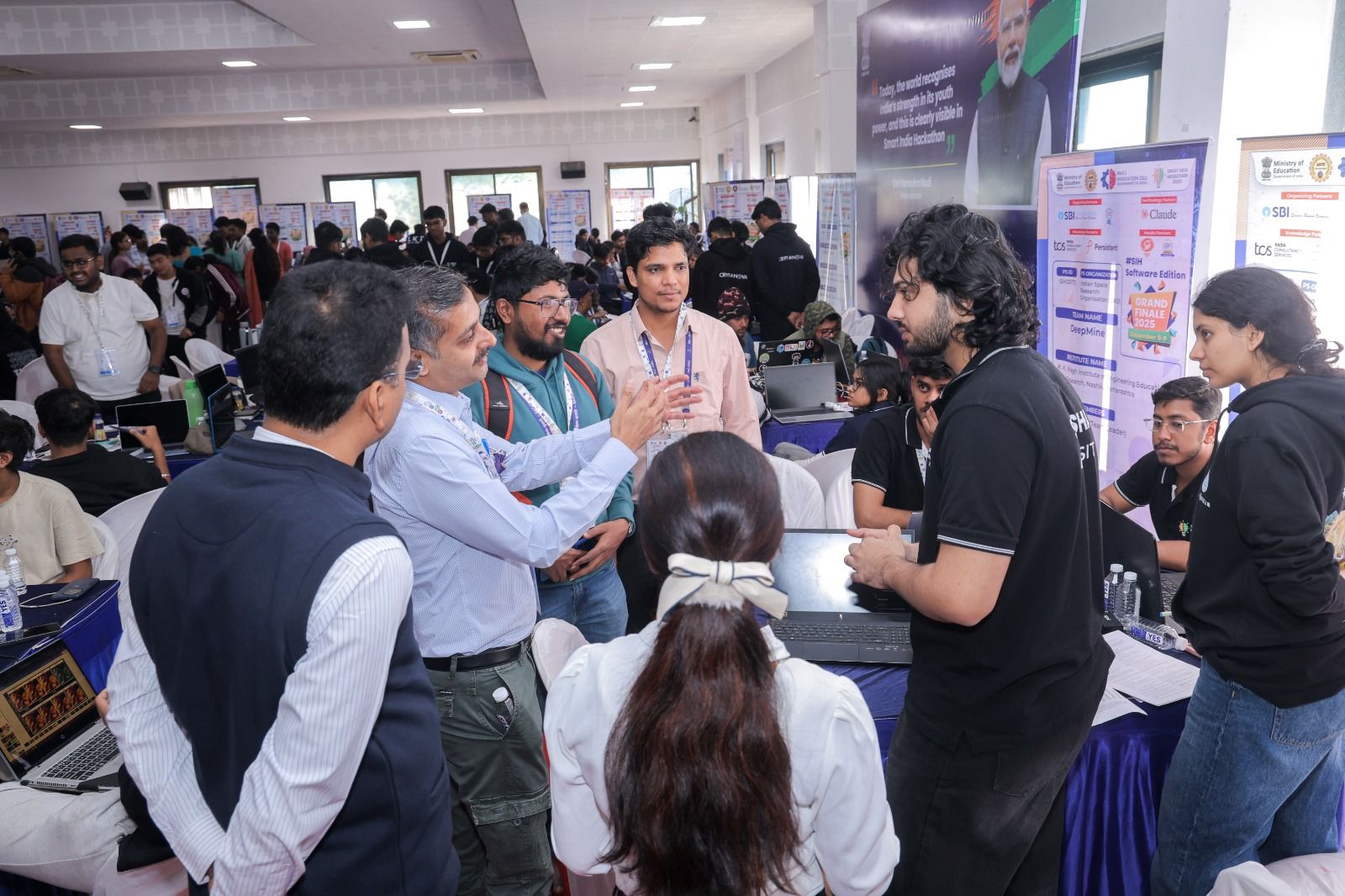
Live discussion round, SIH 2025

Winner announcement, SIH 2025
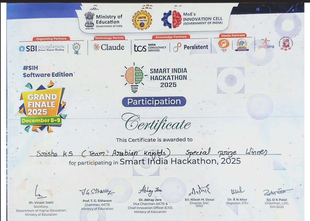
Smart India Hackathon 2025 - Winner Certificate
§1. The Domain & The Problem
ISRO provides Chemistry Transport Model (CTM) forecasts for air pollutants. Forecasting ground-level Ozone (O₃) and Nitrogen Dioxide (NO₂) is hard because they are highly reactive and sensitive to localized weather. Raw CTM predictions had massive biases, often yielding negative R². Satellite data also has huge temporal gaps and measures column density (the whole atmosphere), not ground-level concentrations.
§2. The Mental Model & Trade-offs
Dumping raw meteorological and satellite data into a deep learning model is the obvious first attempt. But standard CV causes massive data leakage in time-series, and neural networks struggle with heavy satellite coverage gaps.
Physics-Informed Approach: O₃ and NO₂ are chemically coupled. A sequential pipeline was the right call:
- Adjust satellite NO₂ using Boundary Layer Height (BLH) to estimate ground-level dilution.
- Predict the true NO₂ concentration.
- Feed that prediction into the O₃ model alongside HCHO as a VOC proxy, mimicking the actual photochemical reaction.
CV: A custom chunk-based Cross-Validation algorithm was written to simulate the exact gap structure of the unseen satellite data (median 24h blind spots).
§3. The Architecture
Data Engine (Polars): Bypassed pandas entirely. Processed 244,000+ time-series samples and generated 200+ complex features.
Domain-Specific Features: Atmospheric physics translated into code:
- Solar Zenith Angle (SZA) and photolysis potentials (J_NO2, J_O3)
- Reaction rates using Arrhenius-type temperature dependencies
- Vertical ventilation and stagnation proxies via wind and BLH
Model (XGBoost): High-capacity GPU architecture (depth 12, 3000 estimators) tuned to capture extreme emission events and penalize false negatives.